손실함수
- 신경망 학습에서 사용하는 지표
평균 제곱 오차(Mean Squared Error, MSE)
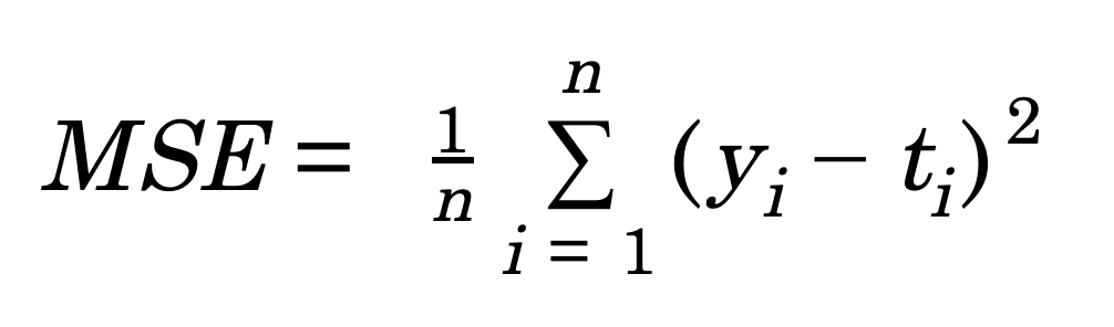
import numpy as np
def mean_squared_error(y, t):
    return 0.5 * np.sum((y-t)**2)
- MSE 값이 작을수록 정답 레이블과의 오차가 작음
교차 엔트로피 오차(Cross Entropy Error, CEE)
- 정답일때의 출력이 전체 값을 결정 (t=1일때)
- 출력값이 커질수록 0에 다가가다가, 출력값이 1일 때 0이된다.(자연로그 그래프)
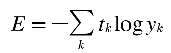
def cross_entropy_error(y, t):
    delta = 1e-7
    return -np.sum(t*np.log(y + delta))
- delta -> np.log 함수에 0을 입력하면 (-inf)가 되어 더 이상 계산을 진행할 수 없기 때문에 작은 값을 더해줌
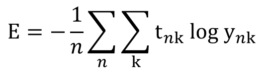
미니배치 학습
(mnist data에 적용)
import tensorflow as tf
def get_data():
    mnist = tf.keras.datasets.mnist
    (x_train, y_train), (x_test, y_test) = mnist.load_data()
    x_train = x_train.reshape(-1, 784)
    x_test = x_test.reshape(-1, 784)

    return x_train, y_train, x_test, y_test
print(x_train.shape, y_train.shape)output : (60000, 784) (60000, )
train_size = x_train.shape[0]
batch_size = 10
batch_mask = np.random.choice(train_size, batch_size)
x_batch = x_train[batch_mask]
y_batch = y_train[batch_mask]
np.random.choice(train_size, batch_size)output : array([44494, 9166, 19148, 21547, 49156, 39646, 6319, 28067, 32994, 29255])
# 레이블이 onehot encoding이 안된 있는 경우
def cross_entropy_error(y, t):
    if y.ndim==1:
        t = t.reshape(1, t.size)
        y = y.reshape(1, y.size)

    batch_size = y.shape[0]
    return -np.sum(np.log(y[np.arange(batch_size), t]+1e-7)) / batch_size
(레이블 Onehot Encoding)
x_train, y_train, x_test, y_test = get_data()
from sklearn.preprocessing import OneHotEncoder
encoder = OneHotEncoder()
y_train = y_train.reshape(-1,1)
y_train = encoder.fit_transform(y_train)
print(x_train.shape, y_train.shape)output : (60000, 784) (60000, 10)
train_size = x_train.shape[0]
batch_size = 10
batch_mask = np.random.choice(train_size, batch_size)
x_batch = x_train[batch_mask]
y_batch = y_train[batch_mask]
np.random.choice(train_size, batch_size)output : array([44494, 9166, 19148, 21547, 49156, 39646, 6319, 28067, 32994, 29255])
# 레이블이 onehot encoding 되어있는 경우
def cross_entropy_error(y, t):
    if y.ndim==1:
        t = t.reshape(1, t.size)
        y = y.reshape(1, y.size)

    batch_size = y.shape[0]
    return -np.sum(t*np.log(y + 1e-7)) / batch_size
손실 함수를 사용이유?
- 왜 매개변수 최적화를 할 때, 정확도 대신 손실함수를 사용하는가?
-> 정확도를 지표로 하면 매개변수의 미분이 대부분의 장소에서 0이 되기 때문
-> 정확도는 parameter의 미세한 변화에는 거의 반응하지 않으며, 그 값이 비연속적으로 변화함(ex. 32%->33%)
(ex)
- weight parameter의 값을 조금 변화시켰을 때, 기울기가 음수일 경우 그 weight parameter를 양의 방향으로 변화시켜 loss function의 값을 감소시킴
- 만약 기울기가 0이면 weight parameter를 어느 쪽으로 움직여도 loss function의 값은 줄어들지 않기 때문에 갱신 중지.
수치 미분
미분
- 한 순간의 변화량을 나타낸 것.
- x의 작은 변화가 f(x)를 얼마나 변화시키는지
def numerical_diff(f,x):
    h = 1e-4 # 0.0001
    return (f(x+h) - f(x-h)) / (2*h)
def function_1(x):
return 0.01*x**2 + 0.1*ximport numpy as np
import matplotlib.pyplot as plt
x = np.arange(0.0,20.0,0.1)
y = function_1(x)
plt.xlabel("x")
plt.ylabel("y")
plt.plot(x,y)
plt.show()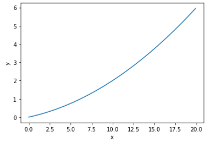
numerical_diff(function_1, 5)output : 0.1999999999990898
-> x에 대한 f(x)의 변화량 = 기울기
편미분
- 변수가 2개이상인 경우에서 미분을 수행할 경우
- 여러 변수 중 목표 변수 하나에 초점을 맞추고 다른 변수는 값을 고정
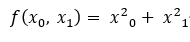
def function_2(x):
    return x[0]**2 + x[1]**2
Q1 x0=3, x1=4일때, x0에 대한 편미분
def function_tmp1(x0):
    return x0*x0 + 4.0**2.0
Q2 x0=3, x1=4일때, x1에 대한 편미분
def function_tmp2(x1):
    return 3.0**2.0 + x1*x1
기울기(gradient)
- 모든 변수의 편미분을 벡터로 정리한 것.
def numerical_gradient(f,x):
    h = 1e-4 # 0.001
    grad = np.zeros_like(x)

    for idx in range(x.size):
        tmp_val = x[idx]
        # f(x+h) 계산
        x[idx] = tmp_val + h
        fxh1 = f(x)

        # f(x-h) 계산
        x[idx] = tmp_val - h
        fxh2 = f(x)

        grad[idx] = (fxh1 - fxh2) / (2*h)
        x[idx] = tmp_val # 값 보원
    return grad
numerical_gradient(function_2, np.array([3.0, 4.0]))output : array([6., 8.]) -> 기울기
- 기울기가 가리키는 쪽은 각 장소에서 함수의 출력 값을 가장 크게 줄이는 방향이다.
경사법(경사 하강법)
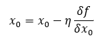
에타 - 갱신하는 양(학습률) -> Learning rate를 너무 작거나 크게 하면 최적의 지점에 도달하지 못함
위의 식을 반복하여 최적의 값을 찾는다.
def gradient_descent(f, init_x, lr=0.01, step_num=100):
    x = init_x
    for i in range(step_num):
        grad = numerical_gradient(f, x)
        x -= lr * grad
    return x
f : 최적화하려는 함수, init_x : 초기값, lr : learning rate, step_num : 경사법에 따른 반복 횟수
ex) 경사법으로 function_2의 최솟값을 구하라
init_x = np.array([-3.0, 4.0])
gradient_descent(function_2, init_x=init_x, lr=0.1, step_num=100)
output : array([-6.11110793e-10, 8.14814391e-10])
-> (-3,4)에서 탐색시작
-> (0,0)에 가까운 결과 도출(실제 정답 : (0,0))
신경망에서의 기울기
weight parameter에 대한 Loss Function의 기울기를 뜻함 -> weight을 조금 변경했을때, Loss의 변화를 봄
import sys, os
sys.path.append(os.pardir)  # 부모 디렉터리의 파일을 가져올 수 있도록 설정
import numpy as np
from common.functions import softmax, cross_entropy_error
from common.gradient import numerical_gradient


class simpleNet:
    def __init__(self):
        self.W = np.random.randn(2,3) # 정규분포로 초기화

    def predict(self, x):
        return np.dot(x, self.W)

    def loss(self, x, t):
        z = self.predict(x)
        y = softmax(z)
        loss = cross_entropy_error(y, t)

        return loss
net = simpleNet()
print(net.W) # weight parameteroutput : [[ 1.14763376 -0.09709734 -1.00984844]
[ 1.34509558 -0.29337843 0.44282171]]
x = np.array([0.6, 0.9])
p = net.predict(x)
print(p)
np.argmax(p) # 최대값의 인덱스

t = np.array([0, 0, 1]) # answer label

f = lambda w: net.loss(x, t)
# def f(W):
#     return net.loss(x, t)
# 이 함수를 lambda로 쉽게 표현 가능

dW = numerical_gradient(f, net.W)

print(dW)
output : [ 1.89916627 -0.32229899 -0.20736952]
[[ 0.48776125 0.05289775 -0.540659 ]
[ 0.73164188 0.07934662 -0.8109885 ]]
정리 및 학습 알고리즘 구현하기
확률적 경사 하강법(Stochastic Gradient Decent)
1. 미니배치 : 훈련 데이터 중 일부를 가져와서 그 미니배치의 loss function 값을 줄임
2. 기울기 산출 : 미니배치의 loss function을 줄이기 위해 weight function의 값을 작게하는 방향 제시
3. 매개변수 갱신 : weight parameter를 기울기 방향으로 조금 갱긴
4. 반봅 : 1~3번을 반복하며 최적의 값 도출
import sys, os
sys.path.append(os.pardir)  # 부모 디렉터리의 파일을 가져올 수 있도록 설정
from common.functions import *
from common.gradient import numerical_gradient


class TwoLayerNet:

    def __init__(self, input_size, hidden_size, output_size, weight_init_std=0.01):
        # 가중치 초기화
        self.params = {}
        self.params['W1'] = weight_init_std * np.random.randn(input_size, hidden_size) #평균 0 표준편차 1의 가우시안 표준정규분포 난수 생성(mxn)
        self.params['b1'] = np.zeros(hidden_size)
        self.params['W2'] = weight_init_std * np.random.randn(hidden_size, output_size)
        self.params['b2'] = np.zeros(output_size)

    def predict(self, x):
        W1, W2 = self.params['W1'], self.params['W2']
        b1, b2 = self.params['b1'], self.params['b2']

        a1 = np.dot(x, W1) + b1
        z1 = sigmoid(a1)
        a2 = np.dot(z1, W2) + b2
        y = softmax(a2)

        return y

    # x : 입력 데이터, t : 정답 레이블
    def loss(self, x, t):
        y = self.predict(x)

        return cross_entropy_error(y, t)

    def accuracy(self, x, t):
        y = self.predict(x)
        y = np.argmax(y, axis=1)
        t = np.argmax(t, axis=1)

        accuracy = np.sum(y == t) / float(x.shape[0])
        return accuracy

    # x : 입력 데이터, t : 정답 레이블
    def numerical_gradient(self, x, t):
        loss_W = lambda W: self.loss(x, t)

        grads = {}
        grads['W1'] = numerical_gradient(loss_W, self.params['W1'])
        grads['b1'] = numerical_gradient(loss_W, self.params['b1'])
        grads['W2'] = numerical_gradient(loss_W, self.params['W2'])
        grads['b2'] = numerical_gradient(loss_W, self.params['b2'])

        return grads

    def gradient(self, x, t):
        W1, W2 = self.params['W1'], self.params['W2']
        b1, b2 = self.params['b1'], self.params['b2']
        grads = {}

        batch_num = x.shape[0]

        # forward
        a1 = np.dot(x, W1) + b1
        z1 = sigmoid(a1)
        a2 = np.dot(z1, W2) + b2
        y = softmax(a2)

        # backward
        dy = (y - t) / batch_num
        grads['W2'] = np.dot(z1.T, dy)
        grads['b2'] = np.sum(dy, axis=0)

        da1 = np.dot(dy, W2.T)
        dz1 = sigmoid_grad(a1) * da1
        grads['W1'] = np.dot(x.T, dz1)
        grads['b1'] = np.sum(dz1, axis=0)

        return grads
net = TwoLayerNet(input_size=784, hidden_size=100,output_size=10)
net.params['W1'].shape # (784, 100)
net.params['b1'].shape # (100,)
net.params['W2'].shape # (100, 10)
net.params['b2'].shape # (10,)x = np.random.rand(100, 784)
y = net.predict(x)x = np.random.rand(100, 784) # 더미 입력 데이터(100장 분량)
t = np.random.rand(100, 10) # 더미 정답 레이블(100장 분량)
grads = net.numerical_gradient(x, t) # 기울기 계산
grads['W1'].shape # (784, 100)
grads['b1'].shape # (100,)
grads['W2'].shape # (100, 10)
grads['b2'].shape # (10,)'Learning > Deep Leaning' 카테고리의 다른 글
| 합성곱 신경망(CNN) (0) | 2021.08.31 |
|---|---|
| 학습관련 기술들 (0) | 2021.08.09 |
| 오차역전파법 (0) | 2021.08.04 |
| Neural Network(Activate Function) (0) | 2021.07.18 |
| Perceptron (0) | 2021.07.18 |


